Task of TCP is to provide a reliable full duplex byte stream in case of connection of best-effort networks between programs operating in the two terminals. Therefore TCP generates a logical connection between the two applications. (As a reminder: IP generates a logical connection between two hosts, while Ethernet generates a physical connection between two neighboring network elements.) TCP means always a connection between two terminals, we cannot realize a point-multipoint connection with TCP. A typical example for this is the connection between the web browser, and the webserver. The two terminals are identified by their IP-numbers, while applications running on them, wishing to communicate with each other are identified by port numbers (with that we mark actually interfaces). This identification is a globally individual one. It is worth to note, that (i) this identifier can change at different points of the transmission route (see also: NAT), and (ii) the individual elements of this identifier are used in differenet layers.
TCP has an influence to the size of the segment, considering its manager functions, making a traffic control and a congestion control. It is important to see, that because of that TCP has a rate/timing/scheduling of data writing and sending, "decoupled" from applications connected by itself. TCP cannot be used properly in case of certain applications because of this - e.g. in case of real-time connections.
TCP generates a connection from a technical viewpoint between the so-called sockets controlled by the operation systems, which can be considered to interfaces from the viewpoint of the application. We can refer to the socket with a port number (see structure of the TCP header below). Operation of a TCP protocol can be divided into 3 parts: (i) generation of connection, (ii) data transmission, (iii) disassembly of connection.
          0                   1                   2                   3
          0 1 2 3 4 5 6 7 8 9 0 1 2 3 4 5 6 7 8 9 0 1 2 3 4 5 6 7 8 9 0 1
         +-+-+-+-+-+-+-+-+-+-+-+-+-+-+-+-+-+-+-+-+-+-+-+-+-+-+-+-+-+-+-+-+
         |         Source port           |      Destination port         |
         +-+-+-+-+-+-+-+-+-+-+-+-+-+-+-+-+-+-+-+-+-+-+-+-+-+-+-+-+-+-+-+-+
         |                      Sequence number                          |
         +-+-+-+-+-+-+-+-+-+-+-+-+-+-+-+-+-+-+-+-+-+-+-+-+-+-+-+-+-+-+-+-+
         |                   Acknowledgement number                      |
         +-+-+-+-+-+-+-+-+-+-+-+-+-+-+-+-+-+-+-+-+-+-+-+-+-+-+-+-+-+-+-+-+
         | TCP   |           |U|A|P|R|S|F|                               |
         |header | Reserved  |R|C|S|S|Y|I|            Window             |
         |length |           |G|K|H|T|N|N|                               |
         +-+-+-+-+-+-+-+-+-+-+-+-+-+-+-+-+-+-+-+-+-+-+-+-+-+-+-+-+-+-+-+-+
         |       Checksum                |       Urgent pointer          |
         +-+-+-+-+-+-+-+-+-+-+-+-+-+-+-+-+-+-+-+-+-+-+-+-+-+-+-+-+-+-+-+-+
         |       Options (if any)                        |   Padding     |
         +-+-+-+-+-+-+-+-+-+-+-+-+-+-+-+-+-+-+-+-+-+-+-+-+-+-+-+-+-+-+-+-+
         |       Data to be transmitted                                  |
                                         .
                                         .
                                         .
         |                                                               |
         +-+-+-+-+-+-+-+-+-+-+-+-+-+-+-+-+-+-+-+-+-+-+-+-+-+-+-+-+-+-+-+-+
According to the issues mentioned above, header consists of at least 20 octets, and we will introduce the individual elements below:
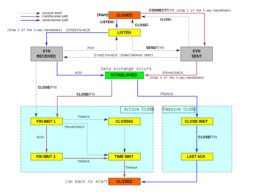
Since TCP connection is a connection oriented network layer protocol, thus before we would like to transmit any data between two applications running on two different computers with the help of TCP, we must build up a connection. Partner initiating a TCP connection is called client host, while the another partner is called server host. Generation of a TCP connection - which is often called 3-way-handshake - is demonstrated on the following figure:
We can read from this figure, that what flags have a value of 1 in the individual segments, and we signed the sequence numbers and sequence numbers of acknowledgements everywhere, where it could be interesting. Initial sequence numbers (ISN) are selected randomly to avoid a possible attack (see in details: RFC 1948).
As it is shown on the figure, we determine the maximum segment size (MSS) by building up a connection, that is the maximum size of data in the application layer at the TCP segment. Measurement of MSS depends on the TCP implementation (that is determined by the operation system), but it can mostly be configured (as it is demonstrated on the figure) with the help of the proper Option header element. Actual value is usually set to avoid the IP fragmentation. IP fragmentation will happen, when size of the IP packet exceeds the maximum size permitted in connection with size of the PDU (Maximum Transmission Unit - MTU). We would like to avoid fragmentation, if it is possible, because it generates an extra traffic in case of resending. That is why value of MSS orientates to MTU. In case of the current Internet IP usually runs over Ethernet (more exactly: we pack the IP packets into EthernetII frames), which have an MTU with 1500 bytes. Certain manufacturers allow the use of the so called Jumbo-frames, and in the case of their usage MTU could even be 9000 bytes, but it may occur only in LANs, and the border protocols (e.g. PPPoE) reducate itt o the common size. In case of a WLAN value of MTU is 2272 bytes. Since TCP generates a connection between two applications running on two different computers, that can be at an optional place in the Internet, we cannot be sure, that the same MTU is valid everywhere during the transmission route. We have to learn the MTU (that will be obviously the smallest MTU) valid for the whole route to avoid repacking en route. This process described by RFC 1191 and RFC 1981, in the case of IPv4 and IPv6, respectively, is called "Path MTU Discovery", and it uses the ICMP.
According to the presently valid recommendations, implementations must support compulsorily the selective acknowledgement (SACK). In this case we use the Option field, and we can acknowledge for one or more coherent range of sequence numbers. This solution improves significantly the efficiency of resending.
Quantity of data being unacknowledged in the network simultaneously is specified by the "Window" (Advertised Window). Destination may tell the resource, how many data it will be able to get, so it prevents, that a fast sender should overrun the receiver (flow control). When packets arrive correctly, in a perfect order, then size of the window is actually constant (or fluctuates only a little bit because of the delayed acknowledgement), but at the same time its beginning point is gradually raising ("sliding? - the name of the window derives from this). We can refer to this self-controlling characteristic with the expression of "self clocking". If packets do not arrive in a correct order, then sequence number of the acknowledgement (or beginning point of the window) is constant, but its size is reducing, because we store packets, that did not arrive in a correct order (if they fall within the window, otherwise we will throw them away). We will also throw the duplicated packets away. This is the way the receiving puffer with a sliding window serves for restoring the sequence of segments. The space of lost parts of the data flow will remain empty in the window. We sign this lack with acknowledgements, and we send a cumulative acknowledgement about the additionally arriving segments, thus the data transmission will be reliable. Usage of Sliding Window is easy to understand from the following figure and formulas.
Conditions of a reliable and ordered data transmission:
Rules of realization of the flow control
Since TCP provides a reliable transmission, we resend every segment, to that does not arrive any acknowledgements within a certain time. We connect a resending timer to every segment, which after the expiration of RTO (Retransmission Timeout) resends the segment. RTO can be determined on the basis of Round Trip Time (RTT) between the two terminals of the communication, however, between two optionally chosen terminals of Internet, RTT can fall into a range covering several orders of magnitudes, and even between two selected hosts generation of delay can show a significant fluctuation in time, so determination of RTT can be a quite difficult task, and there were made better and better solutions over time: :
According to the original algorithm in case of every pair of segments/acknowledgements we measured the actual round trip time (SampleRTT), to that we calculated a weighted amount:
EstimatedRTT = a*EstimatedRTT + b*SampleRTT,
where a+b = 1 and the value of a and b is between 0.8 and 0.9, and between 0.1 and 0.2, respectively.
RTO is chosen on the basis of EstimatedRTT for the following:
TimeOut = 2 * EstimatedRTT
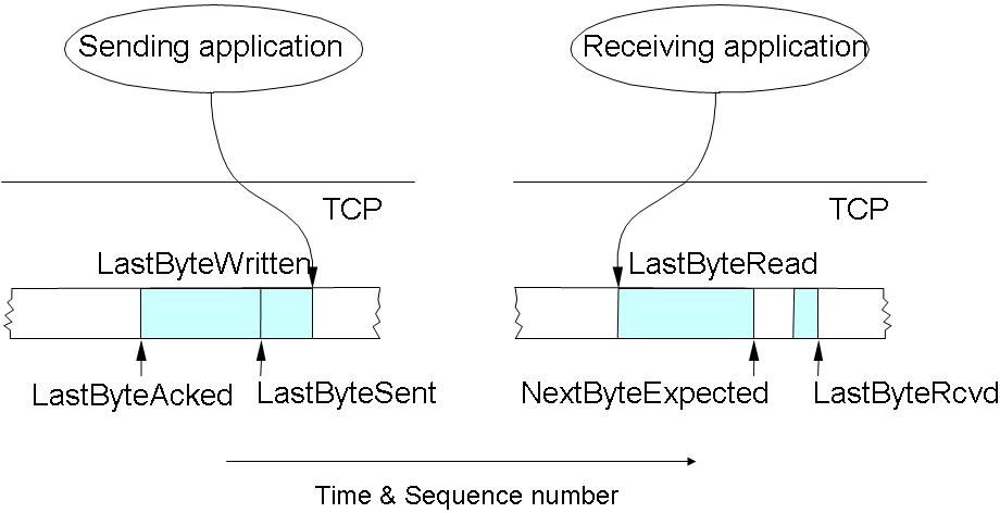
Karn/Partridge algoritm modified the original one, because it was observed, that in case of resent packets SampleRTT does not bear a real information (see the figure below), so we should not take the resent packets into consideration by estimating RTT. At the same time, it generates a further problem, because if we assume a situation, where the transmission delay starts growing significantly very suddenly (between two segments), then the rule mentioned above would mean, that we will not refresh RTT any more. That is why we apply the "exponential backoff", which means, that in case of every resending we will increase RTO twice as large:
new_TimeOut = old_TimeOut*2.
This process provides stability of network in practice.
The Jacobson/Karels algoritm was published first in an article of Van Jacobson in 1988. This article discussed actually more algorithms, that became later official standards, published in RFCs. These algorithms - although they concerned different fields - all recommended solutions for the serial collapses of Internet, beginning from October of 1986. These collapses were caused by congestion (congestion collapse - (C) John Nagle), since standards were not prepared for its handling properly. (As an example, we can tell, that the original algorithm serving for the estimation of RTT was operating approximately till a 30% of loading.) Congestion reduces not only the transmission ability - Jacobson's example: a bandwidth reducing from 32 kbps to 40 bps between two computers, to 400 yard from each other, with 3 IMP hops (Interface Message Processor - network element of ARPAnet) between them -, but it enhances significantly the deviation of the delay of arriving packets. It is easy to understand, that if deviation of RTT is large, then RTO must be significantly higher then the average of RTT. So we will apply the following rules:
Difference = SampleRTT - EstimatedRTT
EstimatedRTT = EstimatedRTT + ( d * Difference)
Deviation = Deviation + d ( |Difference| - Deviation)), where d is a fraction between 0 and 1.
We should take into consideration this spreading by setting RTO:
Timeout = u * EstimatedRTT + q * Deviation, where u = 1 and q = 4 .
Congestion, as we have described it earlier, does not belong to the initial phenomena of Internet, but it was experienced more and more only from the second half of the '80 years. Recommendations for solution have been published in Jacobson's mentioned article. TCP congestion control consists of four algorithms connected to each other, which were described as a standard by RFC 2581. Recently RFC 5681 is valid. There are two new variables occurring in the algorithms. One of them is the "congestion window", which is signed with the "cwnd" (or "CongWin") abbreviation, and henceforth we have to take into consideration the smaller one from the advertised window of the receiver and the congestion window, as a window of the sender. Another variable is the "slow start threshold" (ssthresh), which is a boundary point of the change between the two algorithms. Further important novelty is, that loss of packet is considered to be the sign of congestion, and we react to the loss of packet differently, depending on, if we perceived it on the basis of expiration of the timer, or if we consider it to be lost on the basis of 3 duplicated acknowledgements.
The four processes are the following:
Congestion control of TCP can be considered, as a state machine. The following table informs us about, what kind of transit is possible between the individual states.
| State | Event | TCP Sender Action | Commentary |
|---|---|---|---|
| Slow Start (SS) | ACK receipt for previously unacked data | CongWin = CongWin + MSS, If (CongWin > Threshold) set state to "Congestion Avoidance" | Resulting in a doubling of CongWin every RTT |
| Congestion Avoidance (CA) | ACK receipt for previously unacked data | CongWin = CongWin+MSS * (MSS/CongWin) | Additive increase, resulting in increase of CongWin by 1 MSS every RTT |
| SS or CA | Loss event detected by triple duplicate ACK | Threshold = CongWin/2, CongWin = Threshold, Set state to "Congestion Avoidance" | Fast recovery, implementing multiplicative decrease. CongWin will not drop below 1 MSS. |
| SS or CA | Timeout | Threshold = CongWin/2, CongWin = 1 MSS, Set state to "Slow Start" | Enter slow start |
| SS or CA | Duplicate ACK | Increment duplicate ACK count for segment being acked | CongWin and Threshold not changed |
It is worth to know, that for congestion control occurring at IP networks we have other possibilities not realized at TCP, that, however, are connected to it somehow. These possibilities are, for example, RED (Random Early Detection) or ECN (Explicit Congestion Notification) - we have already mentioned two new TCP signal bits in connection with this later one.
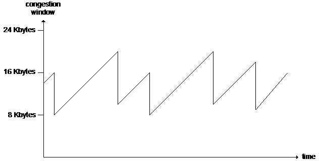
If there is a narrow link shared by several TCP streams, then we may expect, that they should share the resources fairly, independently from the initial parameters. It is provided by Additive Increase/Multiplicative Decrease speed control used at the congestion avoidance as it is demonstrated by the following figure.

It results the well-known sawtooth-shaped speed diagram of TCP, and we can simply estimate the average speed of TCP on the basis of this: 0.75*cwnd/RTT. Naturally, this estimation will only be true, if the congestion window limits transmission and the transmittable byte stream is long enough, that slow start would be negligable compared to the phase of congestion avoidance. The sawtooth diagram characterizes not only the speed, but also its shape can be corresponded to size of cwnd, and to the amount of data in the receiving puffer.
Sequence numbers and acknowledgements in TCP
We must see, that aim of management functions of TCP is to reach the highest possible throughput, exploiting the transmission capacity at our disposal, i.e. we should saturate the link, as far as it is possible. Beyond parts discussed so far, we have to talk about Window and Sequence Number, i.e. about, how can their usage affect the availability of the aim mentioned above.
We have already told about Window, that receiver can send a message to the sender in this header element, and give the number of bytes, that it can receive yet (Advertised Window), which can maximally be 64kBs, because the Window field has 16 bits. Maximum of this size and congestion window gives to the sender, how many unacknowledged data can totally be sent. Let us assume, that receiver has a proper performance, and network is unloaded, and RTT is 50 msecs. It can be simply shown, that resource can only saturate the link, if maximum of AW can be larger, than value of the so-called Bandwitdh-Delay Product (BDP). The following table gives BDP related to values of some possible bandwidths.
| Bandwidth [Mbps] | BDP (RTT=50 msec) [kB] | Time to wrap around |
|---|---|---|
| T1 (1.5 Mbps) | 9 | 6.4 hours |
| ADSL (5 Mbps) | 31 | 1.9 hours |
| Ethernet (10 Mbps) | 61 | 57 minutes |
| T3 (45 Mbps) | 275 | 13 minutes |
| Fast Ethernet (100 Mbps) | 610 | 5.7 minutes |
| STS-3 (155 Mbps) | 946 | 3.7 minutes |
| STS-12 (622 Mbps) | 3796 | 55.2 seconds |
| Gigabit Ethernet (1000 Mbps) | 6104 | 34.4 seconds |
It can be seen, that the line of 10 Mbps can be filled in yet with Window of 64 kBs, but a link with higher rate is not. As a solution for this problem, use Window Scale (RFC 1323) from the options of TCP header: here we have a field of 8 bits, and its value will give, that with how many bits we should shift the received value to the left (and the transmittable value to the right). However, we cannot exploit the gained possibilities: value of the window scale factor can maximally be 14, that corresponds approximately to the window value of 1 GB.
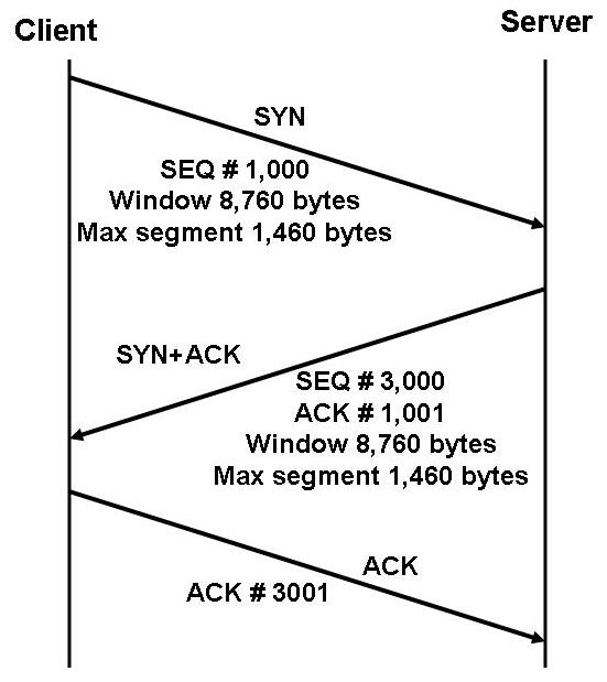
Sequence Number is a rotation number of 32 bits, which has a shift compared to the initial, randomly selected sequence number value, that is equal to the position of the first data byte of a given segment in the transmittable byte stream. Receiver decides on the basis of sequence number of the received segment, whether it fits to the receiver window, or it is must be dropped. We can roughly address data of 4 GBs with 32 bits, that is not very much nowadays. We indicated rotation time measured at the link of a given bandwidth in the 3rd column of the table above (it is the time, when we use the whole set of sequence numbers - time to wrap around). Besides, we have to take into consideration, that windows of the sender and the receiver does not cover each other accurately, so we will learn after some calculation, that it it necessary to keep the SenderWindowSize < (MaxSeqNum +1)/2 condition. As we can see, it happens at larger networks respectively soon. We can search for a solution to this problem among TCP options again. We have a possibility by using Timestap option described in RFC 1323 to distinguish segments arriving with the same sequence number even with a large window size. It is important to know, that timestamp counts time units, and we can initialize and synchronize the counter during SYN-SYN/ACK messaging. We have to use in connection with the selection of timebase values between 1 msec and 1 sec according to the standard. Sometimes a timebase between 10 and 100 msecs is selected in practice. It is proper for using Timestamp option for another purpose, because we have also a possibility with sending back the timestamp to measure RTT respectively accurately. We can use result of this measurement for both the calculation of RTO, and for the forecast of congestion.
We can obtain an expressive image about characteristics of the given TCP stream, plotting TCP sequence numbers as a function of time. We can track not only the individual steps of congestion control on a correctly scaled diagram, but also we can read the characteristic amounts related to the connection of TCP (e.g.: MSS, RTTs, RTO, window sizes, etc.).

We have to close the connection after transmission of the last byte of the TCP data stream. This closing consists of segments with FIN signal bits and their acknowledgements sent mutually by the two parties, so we use basically 4 message, which is not surprising, if we think about, that TCP provides a full-duplex connection. The following figure demonstrates a possible case. It is worth to note, that we will not get into a CLOSED state immediately after the second acknowledgement in the state graph, but we must wait for the expiration of a timer.

We can read from the figure, that it may occur sometimes, that one of the parties has already closed the connection, while it was open from the other side (half open). It may also happen, that the two parties intend to close the connection mutually, so both of them send the FIN segment without getting this kind of issue from the other party. Finally we have to mention, that it is often used in today's implementation the proper version of TWH, which means, that the acknowledgement given to the active FIN, and the passive FIN are in the same segment.
Continuous growing of the network bandwidth raised the problem of saturation of the link, which has already been mentioned earlier, and another problem, that time of feedback (RTT) can be comparable with time necessary for reception of the whole file in case of smaller files, however, it will be significantly longer, than it would be necessary because of the slow start. It results, that congestion control and traffic control will not be efficient, and exploitation of the link will be small. We have already demonstrated some possibilities above, with that we can exploit more transmission provided by high-speed networks, but many people think, that we need new algorithms instead of trying to improve TCP. The following table demonstrates some more known of the so-called high-speed TCP-variants.
| Name of protocol | Type | Who and when recommended it | Main features |
|---|---|---|---|
| HighSpeed TCP | based on packet loss | S. Floyd, International Computer Science Institute (ICSI), Berkeley University of California, 2003. | AIMD |
| Scalable TCP | based on packet loss | T. Kelly, CERN & University of Cambridge, 2003. | MIMD |
| BIC TCP / CUBIC | based on packet loss | I. Rhee et al., Networking Research Lab, North Carolina State University, 2004. és 2005. | good throughput, fairness, and stability |
| FAST TCP | based on delay | S. Low et al., Netlab, California Institute of Technology, 2004. (ma: FastSoft Inc.) | promising fairness features |
| TCP Westwood | measurement based | M. Y. Sanadidi, M. Gerla et al., High Performance Internet Lab, Network Research Lab, University of California, Los Angeles (UCLA), 2001 és 2005 között | more variations, different estimation methods |
| Compound TCP | hybrid | K. Tan et al., Microsoft Research, 2005. | AIMD + delay based component |
| XCP | explicit congestion notification | D. Katabi et al., Massachusetts Institute of Technology (MIT), 2002. | it is necessary to modify routers |
UDP is a user datagram protocol. It provides for the users to send messages without setup and tear down of a connection. It does not guarantee either delivery of messages, or keeping their order.
          bytes (20)   from IPv4 frame
              +--------------------------------+
            2 | Source Port                    |
              +--------------------------------+
            2 | Destination Port               |  Pl: 5004 (avt-profile-1) RTP media data
              +--------------------------------+
            2 | Length  (8 byte header + max.  |
              |          65527 byte data)      |
              +--------------------------------+
            2 | Checksum (header+data)         |
              +--------------------------------+
0000  70 cd 70 64 08 00 45 b8                           ..)../.`p.pd..E.
0010  00 c8 9e 11 00 00 3e 11 c1 48 98 42 f5 ab 98 42   ......>..H.B...B
0020  f5 e2 46 b0 13 8c 00 b4 00 00 80 00 3d 7c 00 28   ..F.........=|.(
0030  0c 40 d4 7b 28 21 f9 f7 fc ff 7b 7d fd 7c 7c 78   .@.{(!....{}.||x
0040  7a fc 7c 7a 7f fd fd 7e ff fd fb f8 f3 f0 f3 f7   z.|z...~........
0050  fc fb f8 fa 7d 76 78 79 77 77 78 7a 7b 7b 7c 7d   ....}vxywwxz{{|}
0060  7e fe fe fd f9 f7 fb fc f7 f9 fb fb fc fa fa fd   ~...............
0070  fd fb fb fa fd fe fd fc f8 fa fd fb fc fd fb fa   ................
0080  f8 f8 fe fe fa fa fb fd 7e 7b 79 78 79 7f fa fe   ........~{yxy...
0090  7c 7f 7e 7c 7e 7f 7b 7b 7c 7a 78 78 78 74 75 79   |.~|~.{{|zxxxtuy
00a0  7c 7c 7c 7f fc f9 fa fc fa f9 f9 fc 7d 7e fb f9   |||.........}~..
00b0  f7 f9 7f 7e fe fd fb fb fc fe 7d fc f9 fe 7e 7b   ...~......}...~{
00c0  7c 7b 7b 7a 79 7b 7a 7c 7c 79 7c 7a 79 7b 7c 7b   |{{zy{z||y|zy{|{
00d0  7b 7b 7b 7c 7b 7b                                 {{{|{{